Return to Home, Goto Next Section
And just for fun, Navy mechanical computing training spotted by Randy Thelen
This information is grouped into the following sections:
- History of the Nike Analog Computer
- Mission of the Nike Computer
- What is an Electronic Analog Computer?
- Nike Hercules Analog Computer,
- Nike Digital Computer (installed after 1975)
- Solving the Predicted Intercept problem
- Missile Guidance Summary
- Steering Command Details
- About the Nike Plotting Boards
- How does the computer know the radar offsets?
- Gotta have a little fun - Mechanical computers.
- The Surface to Surface mission/mode
From FM 44-1-2 ADA Reference Handbook, 15 June 1984, see page 21 "Rings of Supersonic Steel"
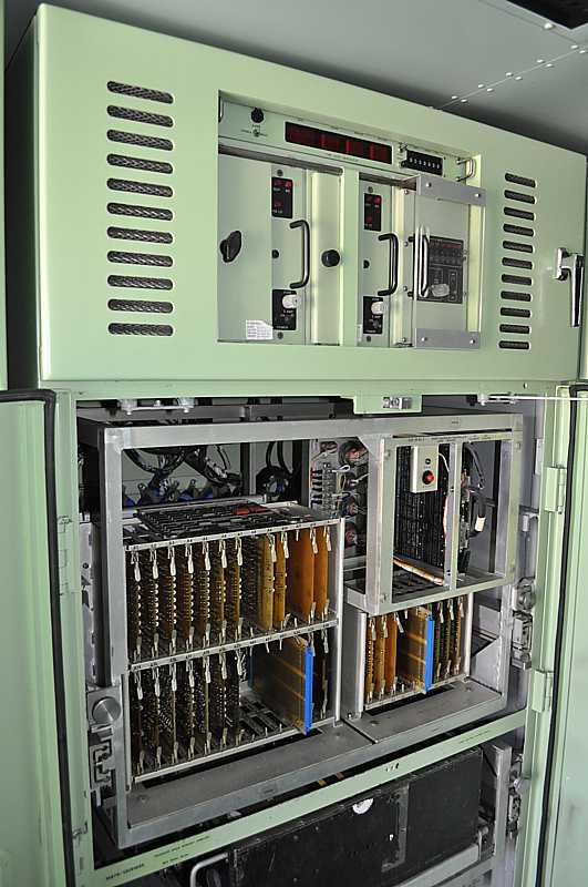
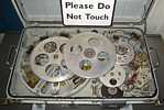
| Nike computer -
Installed in class room, not BC van.
From Rolf Goerigk
|

|
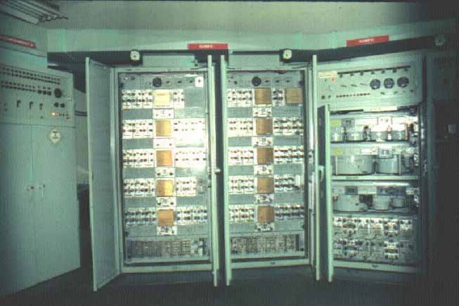
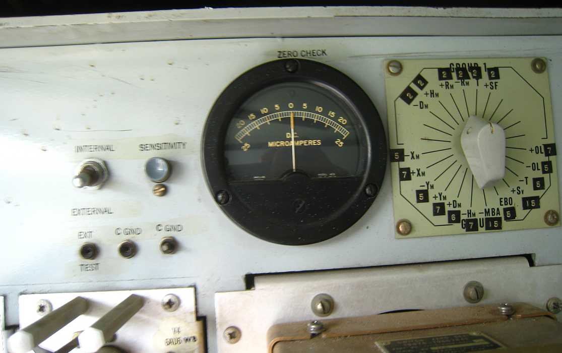
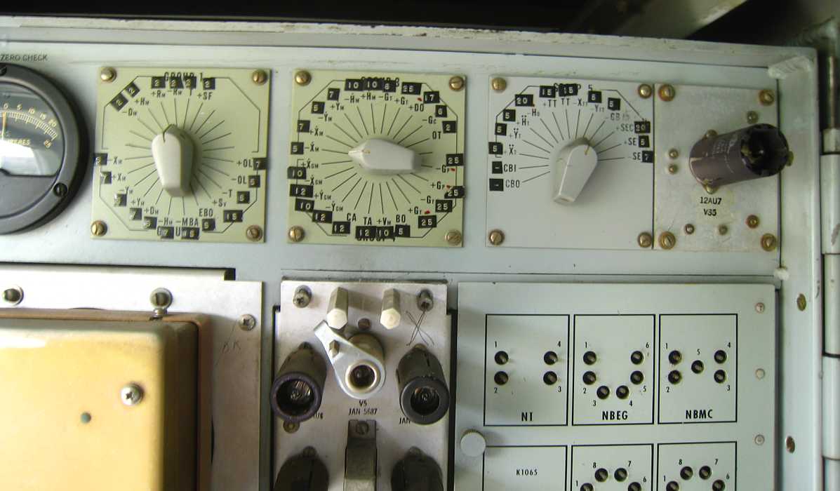
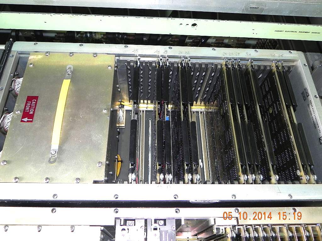
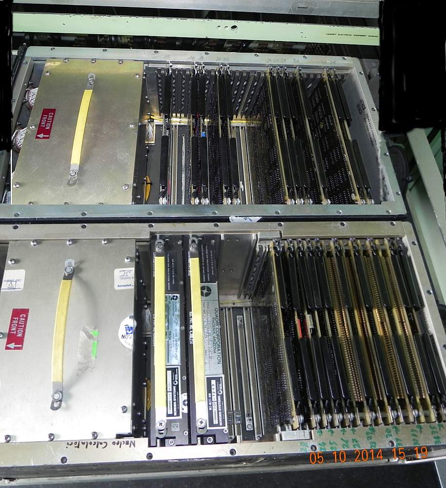
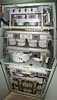
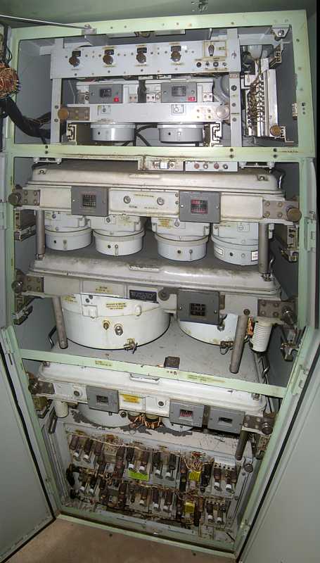
So - the Nike Analog Computer System
- this is one of four cabinets or racks - includes Zero Set Switches (the brown boxes) each can zero set 12 operational amplifiers. |
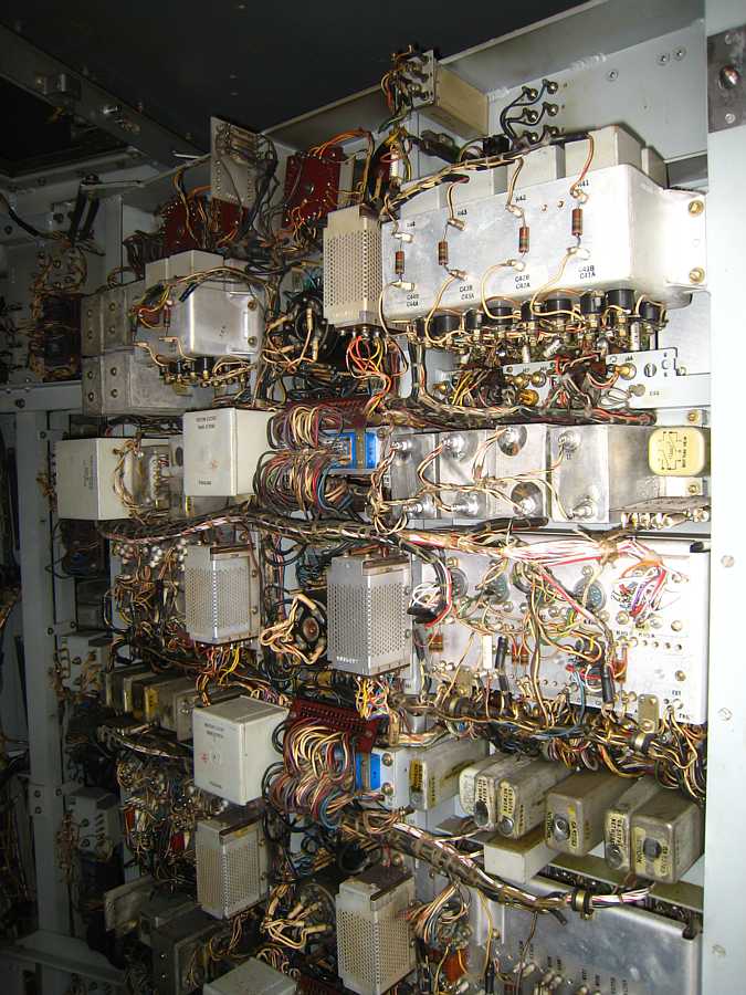
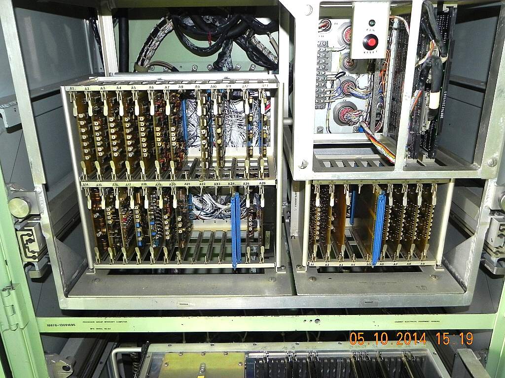
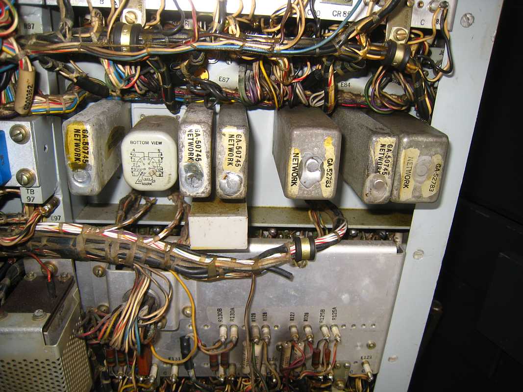
| Back of a swing out door/rack. Lots of components - Analog computers of this complexity, 78 Operational Amplifiers, were expensive and heavy. Look at all that hand wiring and soldering. Days of work - Your cell phone likely costs less than many of the components you are looking at - |
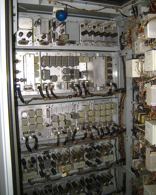
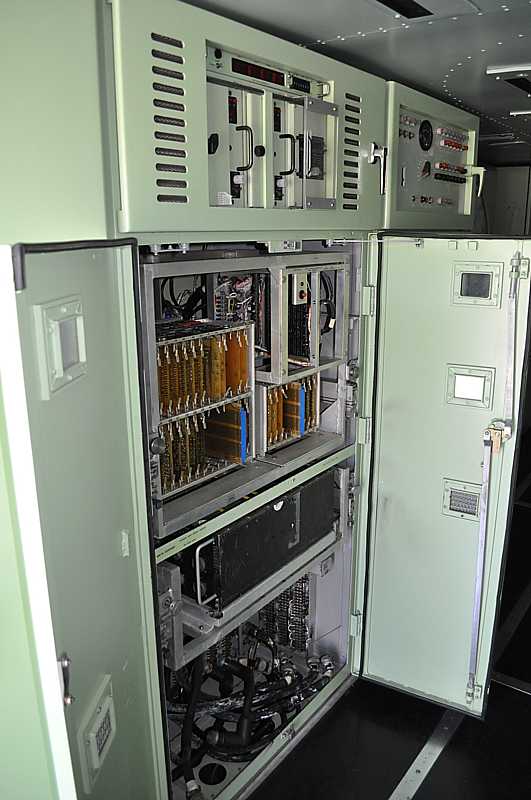
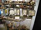
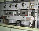
| The wall behind a swing out door. Note the many relays to set:
- operational modes, pre-launch, launch, 7 g dive, 1/2 g cruise - and many test conditions, known inputs to get known outputs |
0) History of the Nike Analog Computer
Now that digital computing logic elements (transistors) are- how many thousands per penny? - and floating point pretty much eliminates scaling,
Digital computing has pretty much taken over from Analog computers for process control.Back in the goode olde dayze,
- beginning before the 1930s and Vannavar Bush's differential analyzer at MIT http://web.mit.edu/klund/www/analyzer/ - until the 1960s
Analog Computing was the practical process control for the masses.- Not many could afford the ENIAC, - or the other massive vacuum tube collections. - And a few hundred tubes are a lot more reliable than thousands. In the late 1930s, mechanical computing elements
- with rather awkward torque amplifiers to handle gain, friction and losses - began to give way to electrical computing elements with vacuum tube amplifiers to handle gain, resistance and losses So - at the beginning of WWII, the needs for solving dynamic fire-control problems
began to be solved by electronic analog computers. http://www.ed-thelen.org/pre_nike.html#gun_dir http://en.wikipedia.org/wiki/Operational_amplifier#1941:_First_.28vacuum_tube.29_op-amp
[Note: most artillery people did not have time to reference the printed fire control tablesgenerated by human computers or by ENIAC.
The tables were needed to generate- cam configurations - potentiometer tapers
for the analog fire control computers. ]
A few generations later (1950), with improvements
(including automatic rather than manual analog amplifier zero setting :-))
the M-33 analog fire control computer for anti aircraft guns was in the fieldand working well - So, by the time the Nike missile system was needed, (1950)
the computing and display elements of the M-33 were used for the related missile guidance problem. Actually, there was practically no choice, digital computing technology would not catch up/supercede analog for many control functions for about 20 another years. In 1974, when most of the Nike systems in the US were being shut down, a digital computer replacement (a militarized DEC PDP-11) was replacing the Nike analog computer in the rest of the world.
1) Mission of the Nike Computer
The Nike Computer had the following main missions:
- a) Provide Predicted Intercept Point and Predicted Flight Time to Plotting Board - for human viewing
- b) Provide Predicted Intercept azimuth angle to missile during pre-launch
- c) Provide Missile Steering commands after launch
- d) Provide Missile Burst command at correct time after launch
- e) (The Nike Hercules Computer had an added Surface-to-Surface function.)
- f) And of course be easy to test, highly reliable, accurate, testable and maintainable
- g) - and be compact enough to fit into a van with other equipment and functions.
There were three main modes:
- Test
- Pre-Launch - Compute Predicted_Intercept_Point and Time_of_Flight to plotting boards
- Post-Launch - add Missile_Steering and Burst commands
a) The Predicted Intercept Point is the point where the missile would intercept the aircraft if:
- the aircraft continued in a straight path and at the same speed
- the missile was fired right now
and the Predicted Flight Time is the time from now for that meeting.
Before launch, this information is useful for the human decision making about when to fire a missile.
After launch, this information is continuously updated based upon actual aircraft flight and missile position and flight characteristics.b) The Predicted Intercept Azimuth is the direction from the launcher to the current Predicted Intercept Point. This direction (azimuth) was sent to the gyro in the selected missile before launch, and was used to provide the missile a sense of "down". This missile gyro and the missile control system kept the belly of the missile "down" and provided the computer and missile a common sense of "down" and left/right.
c) During missile flight, the computer sends Steering Commands to the missile (via the missile tracking radar) to guide the missile to the continuously updated Predicted Intercept Point.
d) The Missile Burst Command is generated by the computer since:
- A human is much to slow and variable to send the command. Since the missile is traveling at about 3000 feet per second, a 0.1 second mistake means a missile explosion 300 feet from the intended location (a clear miss).
- Nike missiles did not "see" the intended target, and could not generate their own burst command. (Although they would automatically burst if they did not receive steering commands for 2 seconds.)
The Missile Burst Command is sent via pulse codes through the missile tracking radar. e) And of course be highly reliable, accurate, testable and maintainable.
In the 1950's, digital computers had tens of thousands of vacuum tubes, and because the vacuum tubes had a mean time to failure of only a few thousand hours, the computers had a mean time to failure of only a few hours. 90 percent "up" time was considered outstanding, and required a round the clock staff of real experts. Digital input and output devices were similarly failure prone. (In the 1970s, when reliable transistors and integrated circuits, and cheaper high speed memory became available, some Nike analog computers were replaced by digital computers.)The only alternative that was reliable enough and accurate enough was the electronic analog computer, which could be implemented for the Nike with fewer than 500 vacuum tubes. There were failures, but the technology was maturing, the tubes were run in a different (not ON/OFF) manner, and the uptime exceeded 99% at most sites. (One failure a month was considered really poor.)
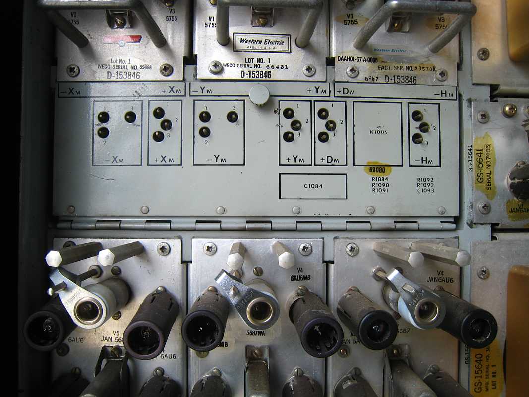
These test points are inputs to computing networks, easily accessable. A "Null Voltage Test Set" could be plugged into these test points, and was sensitive to 1/400 volt ( 2.5 millivolts ) 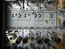
Some of the built-in test and trouble shooting aids 
(In the late 1970s, the analog computer was replaced by a digital computer, a PDP-11 W (running the RT-11 operating system. Two of the 4 analog computer cabinets became closets and storage space.)
2) What is an Electronic Analog Computer?
The Nike analog computer was single purpose, a fixed program with a few different modes set by relays to simplify and automate testing and different modes of operation.
wikipedia Analog_computer
An interesting Analog Computer Web site Reverse-engineering precision op amps from a 1969 analog computer
Another Bernd Ulmann's Analog Computer MuseumSchematics and Operation Manual for the Heathkit EC-1 here
From "The Analog Computer Museum and History Center" - no longer available
Analog computer - A computer that performs mathematical operations in a PARALLEL manner on CONTINUOUS variables. The components of the computer are interconnected to permit the computer to perform as a model, or in a manner ANALOGOUS to some physical system.
Electronic analog computer - An analog computer with input, output and program operations that are usually expressed in terms of direct current voltages.
Analog computers may seem to be "simple" or "like a toy computer", in fact they are powerful tools that were used during the 1950s and 1960s to design and test systems like ICBMs, supersonic aircraft and spacecraft. But the analog computer can be used to model any physical system that can be described by mathematical formulas, even more mundane ones from modeling the effects of pollution on the fish population in a river to fine tuning the suspension on a new car design. Analog computers will not only test a fixed design but also allows variables to be quickly changed to test "what if' conditions. By scaling time as an independent variable, physical processes that happen quickly can be stretched out, and processes that happen over a long period can be shortened to make the process easier to study. And it is very easy to study variables at any point in the program while it is running to find faults in the program design.
Although the analog machine is correctly termed a computer, it does not perform its computations by numerical calculations as does the calculator or the digital computer. The analog computer performs mathematical operations on CONTINUOUS variables instead of counting with digits. Positive numbers are represented by positive voltages and negative numbers are represented by negative voltages, all scaled to the computer's working range, usually -100 volts to +100 volts (vacuum tube) or -10 volts to +10 volts (transistorized), Thus the analog computer does not subtract 20 inches from 45 inches to obtain 25 inches but, rather, it subtracts 4 volts from 9 volts to obtain 5 volts. This 5 volts the operator reads as 25 inches in accordance with his arbitrarily specified "scale factor' of 1 volt equals (or is ANALOGOUS to) 5 inches.
The analog computer is basically a set of building blocks, each able to perform specific mathematical operations on direct current voltages and capable of being easily interconnected one to another. Some of the basic operations include addition, subtraction, multiplication, division, inversion, and integration. By interconnecting these building blocks, mathematical equations are modeled. BUT an analog computer is a true PARALLEL computer that can solve one or one thousand equations at the same time. In fact, similar analog computers can be easily connected together to increase their computing power. When you think about the result of many equations being solved simultaneously and becoming the input to other equations, and sometimes these solutions are then fed back or looped back into the original equations with all of the variables changing CONTINUOUSLY with time, then you can get a brief glance into the incredible power of these computers. Output is usually a voltmeter, oscilloscope, or plotter.
Many universities today like Massachusetts Institute of Technology, University of Illinois, University of Notre Dame, and Purdue University offer classes or do research using analog. computers, because they realize that the last chapter of the history of analog computers has not being written. It's an ANALOG universe and analog computers are a natural way to study and understand it.
Prepared by:
We do except donations of your unused analog computing equipment, working or not.
- The Analog Computer Museum and History Center
http://www.cowardstereoview.com/analog/">http://www.cowardstereoview.com/analog/ - no longer available
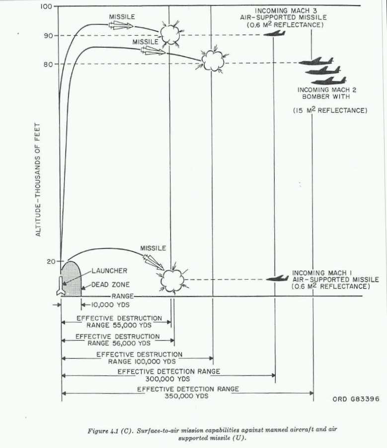
The "Improved Nike Hercules" computer commanded the missile flight in several selectable modes (see MMS-150 Chapter 1)
Surface to air mission - against high and medium altitude targets. Initial dive (from almost vertical), then 0.5 g path to predicted intercept point. (Same as the Nike Ajax computer mission above.) 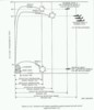
from TM9-1400-250-10-2- Surface to air low altitude mission - against low altitude aircraft - the missile sustainer motor start is delayed to obtain a lower altitude of the boosted part of the flight path. Able to attack closer low altitude aircraft. Uses a "climb-and-dive" trajectory to minimize "the effects of ground clutter in the missile tracking radar system."
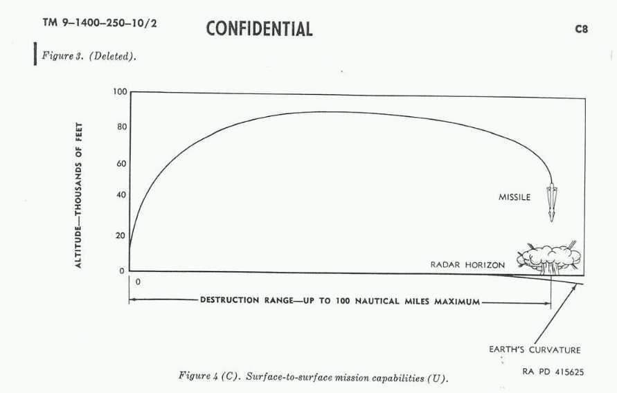
Surface to surface - attack surface targets below the radar horizon. Dive straight down on a stationary target. The burst order causes guidance cutoff rather than an explosion. 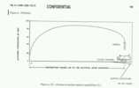
from TM9-1400-250-10-2- Radar scoring for Air Force simulated bombing runs.
From the deployment of Nike in 1954 to the mid 1970's, the Nike Computer was an analog computer. That means that distances, times, and other values were not digital bit representing numbers (like 12.3) but were (in this case) voltage values (like 12.3 volts).
The values as stated above were voltages, and simple circuits (using 76 "operational amplifiers" of 2.5 tubes each) could quickly (1 microsecond):
- add or subtract 2 or more variables
- determine rate of change (of distance giving velocity)
- multiply or divide a variable by a constant
- approximate a function to 1 %
but slower motor driven potentiometers were required to: Each amplifier had a nominal gain of 20,000
- multiply or divide a variable by a variable
- store a variable for a long time (minutes or hours) (not needed in anti-aircraft)
- generate a precision non-linear function
- most amplifiers used "semi-precision" zero set switches with gains of 200, giving effective gains of 4 million.
- about 6 amplifiers used "precision" (re-entrant) zero setting, with gains of 3,000.
There were 2 operational amplifiers using a total of 5 tubes on a chassis. The output tube was a dual triode, 1/2 of the tube was the final amplifier for an amplifier. The "plate" (where the electrons landed) of the final amplifier could be swung between -100 volts and +100 volts using the required external load resistor.
Chassis
DetailFurther details on the operational amplifier are in the Technical Manual TM9-5000-13-Ch03 DC Amplifier Circuitry 265 KBytes
For images of the motor driven potentiometers see Computer (Servo driven potentiometers) and Computer (Details of Time Potentiometer)
The Nike anti-aircraft problem did not require many slow motor driven circuits (about 7) and used about 100 of the simple fast circuits. It also used numerous relays to change between the various modes of operation (test, pre-launch, post-launch). An interesting characteristic of analog computers is that the circuits tend to run in parallel, The relatively slow circuits all working together easily keep up with the anti-aircraft problem in real time.
An analog computer (distances and times were voltages) used analog (voltage) inputs from the Target Tracking and Missile Tracking Radars.
These values (and derived target and missile velocities) were used to calculate the remaining flight time and Predicted Intercept point. The missile was guided to the predicted intercept point by the computer generated steering commands sent through the Missile Tracking Radar.
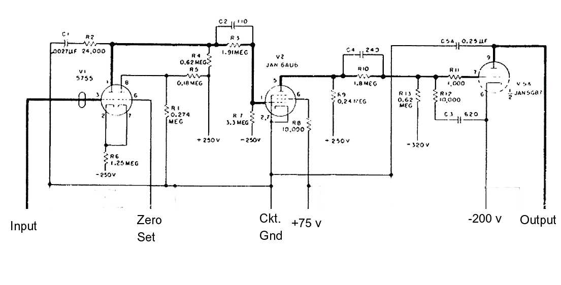
For vacuum tube enthusiasts, here are schematics of a
- operational amplifier (42 K bytes) - power supply - voltage reference - + 450 volt 1 amp thyratron power supply
used in the Nike Ajax and Hercules (as well as the earlier M-33 gun laying analog computer and radar system).The Nike analog computer did not use integrators, but did use filtered differentiators for velocity determination as well as motor driven potentiometers for multiplying by a variable (including time to intercept) as mentioned above.
Another system of amplifiers and motor driven switches performed as "Zero Set Amplifiers" to:
- zero the bias of the operational amplifiers
- increase the effective gain of the associated operational amplifier(s) (to over 1,000,000)
- alarm on excessive inputs caused by operational amplifier failure or computer not settled to a valid "answer".
A number of preset test cases (switch selectable) helped assure that the computer was performing correctly.
Manual knobs input the offset between the missile tracking and target tracking radars. (For further information, you can jump ahead to 6) How does the computer know the radar offsets?

4) Computer Upgrade to Digital
Click here for the digital computer itself
Nike System upgrade to digital
Ramiro CARLI BALLOLA wrote Sept 19, 2015
Hello to everybody, I'm starting answer your questions received by your mail dated September 17, This is the story, first of all in 1959 the first system was deployed in Europe, 8 Countries were participating under the MAP , in 1961 the Logistic support was placed under the control of NAMSA (a NATO maintenance Agency) and the first NIKE Support Conference (SC) among 8 Countries plus the Firing Range in Crete (Greece) was held and followed by other 17 SC.
- No problems with the pictures and message (the pictures I'm sending are mine)
- To answer to all other questions is preferable that I list a sequence of modification (and what the MWO introduced into the system) implemented on the European Nike Systems after the U.S. phase out in 1974.
In 1973 MICOM (Missile Command) changed the assistance conditions and a new agreement was taken with NAMSA to ensure the technical and supply assistance until 1985 with NAMSA.
In 1977 the Support Conference was changed in WSPC (Weapon System Partner Ship) to take control of all aspect (supply, maintenance, overhaul ecc...) of the system support in Europe, still under MICOM external assistance.
MICOM assistance for the nuclear parts was directly followed until 1988 (when the nuclear warheads have been dismissed from the European Systems).
Starting from 1985 all Maintenance aspects was taken directly from NAMSA, transfer of know how took place except for the Engineering parts from 1985 to 1988, after that also the engineering parts were released and the European facilities started the direct assistance in 1989, acting to maintain the system capability until 2005 for ITALY-GRECE and TURKEY (all other 5 countries were phasing out their systems).
Since 1977 started the studies by AT&T for the main and relevant modification to bring the system to be converted in Solid State NIKE Missile System.
As you know the universal Nike System was really universal until the SAMCAP mod. in 1972 (implemented in Europe from 1973 to 1977)
This was a big change because introduced the first solid state circuits into the system. (the first change with the transistors addition was made by the LOPAR AJD modification in the period 1963-1964).Starting from the SAMCAP baseline the RAEMOD (Range and angle encoder modification) prepared by SIERRA RESEARCH CORP. was implemented into the systems and consisted in the following changes:
After the implementation of the RAEMOD from 1978 through 1983 took place another big modification called NAMSA NIKE Support Plan to bring the hybrid system to be completely digital.
- For all tracking antennas, Azimuth and Elevation sin-cos old pots modified and converted to digital output by the mean of opto-electrical converters, (no more Bayol D change and spilling and heavy pots to be moved)
- Range pot completely taken out and changed with the new box (heavy like the old one) containing 4 mini computers for the TTR:
Other three mini computer for the MTR, the difference was that AES-RTS-PCS had the same function of the TTR, but instead of the CCS was only a buffer circuit to transfer the data to the TTR CCS which output was composed of 12 digital words (representing the radar coordinates) to be sent to the computer.
- AES Angle Encoder Section (converting azimuth and elevation info to az/el error signal for the mechanical tracking and to a digital words for the computer)
- RTS Range tracker section (converting the range info to a signal for tracking the target and to a digital words for the computer)
- PCS Periferal controller section to transfer all the signals to the appropriate circuits still inside the pot.
- CCS Coordinate Converter Section (to convert az-el-rng from geographical [or polar] to rectangular coordinates) this circuits were working for the MTR too.
- Because at that time the computer was still analog (except the Zero Set switches converted to solid state) a new item was implemented located into the computer power supply section, the CCDA (Coordinate Converter Digital to Analogic) called also (RCU (Radar Conversion Unit) to bring the 12 digital words back to analog info to be used by the analog computer.
This was a very delicate and unstable circuit due to the thermal control of the converting networks inside, but was only to cover the gap until the introduction of the digital computer in the 80's.
The modification was composed of:
Tracking Antennas
TTR/MTR antenna to be digitalized changing:Bore Site Mast
- TTR/MTR the old TR Electron Tube with a new TRL (Transmit-Receive and limiter)
- TTR only, adding a new Imageless rejection mixer and new converter with solid state amplifiers.
- TTR/MTR changing the old klystron local oscillator with a new VTO (still oscillator voltage controlled)
- TTR/MTR new solid state Skin AFC (automatic Frequency control)
- TTR/MTR new Coaxial Magnetron to have more stability
- TRR new Power Monitor, new duplexer with a new type ferrite switches, TRL's and solid state amplifiers
- TRR new solid state Tracking data's
RC Van
- R.F.T.S. (Radar Frequency Test Set) completely converted to digital at the same time of the other MWO's to bring the NIKE to digital system. Used for test purposes for TTR/MTR/TRR.
Inside the RC Van we had the remote control of the RFTS.BC Van
- TTR new solid state Synchronizer, Video Time Share Amplifier, Lin-Log circuits, IF Amplifiers, LP and SP filters, Video and AGC amplifier, Beacon AFC, Az/El error converter, Az/El angle amplifier, IF test signal generator, Remote RFTS control, Signal strength meter, B scope amplifiers .
- MTR new digital Hercules Coder, same modification as for the TTR except Synchronizer and LP filters
- Completely new digital Track Data Processor, able to analize the 12 words coming from the TTR CCS and performing local simultaneous test (at that point in time all the radar tests were terminated) other than radar parallax conversion for all three radars.
- TRR new solid state IF test signal generator, IF amplifiers and ancillary circuits
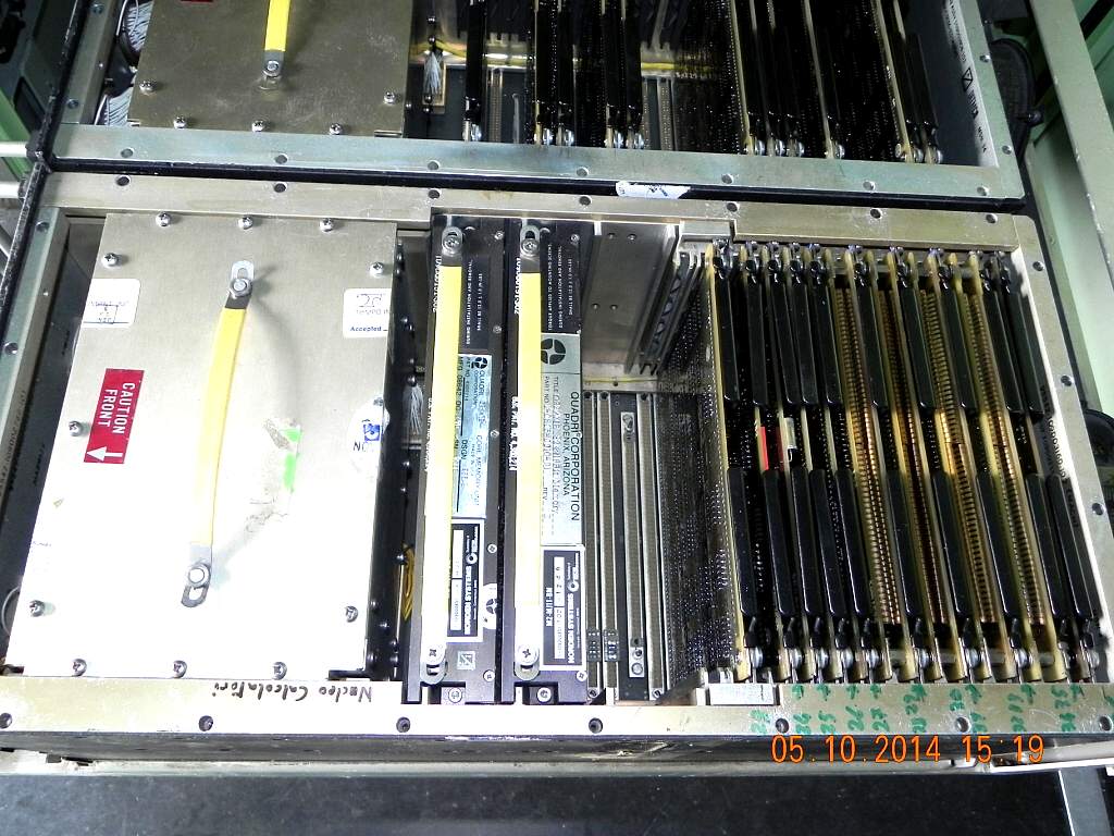
Resulting layout of the previous analog computer area ( From Ramiro Carli Ballola, Feb 2022 )
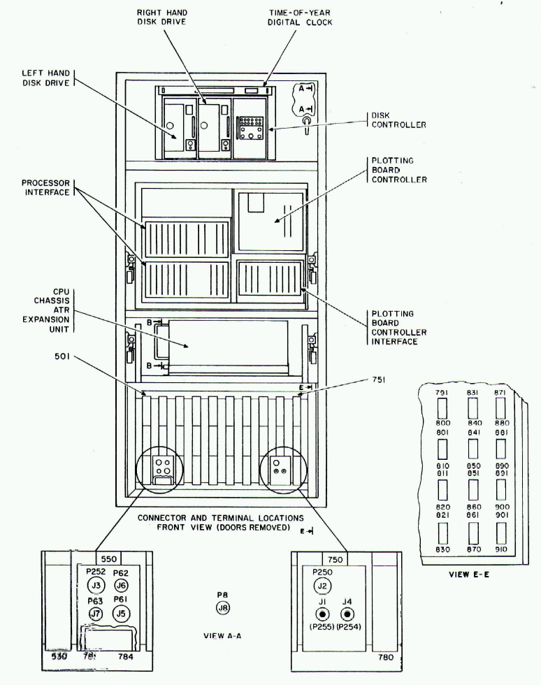
- New digital computer DEC PDP 11/34, located in the former old pot's bay) and supply bay, the first two bay have been left empty (used after many years to include the new IFF system) composed of:
Former pot's bay
- two boxes containing CPU and Expansion circuits
- Intercept computer controller for the Plotting boards (with another mini computer) and all circuits relevant to the incoming info by the radars and from the computer to the Launching area.
- 2 Floppy disks (8 inches) one to record the Missions and the other one with the Tactical disk containing the computer program, one controller and one real time clock, there was another disk containing the computer diagnostic software.
Supply Bay
- Digital Display
- Digital keyboard
- Thermal printer
- New digital Tactical Control indicator
- New plotting boards arms movements by means of stepping motors and new pen type
- New complete Digital AJD circuits
- New digital STC amplifier, az/rng amplifier circuits, PI and PPI all circuit at solid state
- Inside the Director Station Group all circuits converted to digital circuits plus a completely new DMTI (Digital Moving Target Indicator)
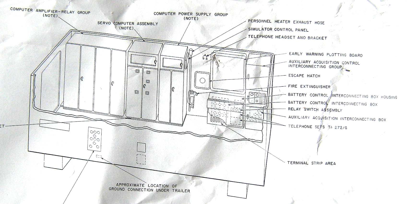
- for your reference, the previous analog computer bays are depicted here.
Starting from BC Van entrance door,
- the first two bays on the left side, has been used to insert the new IFF/Mark XII with Mode 4 system installed years after the computer digital implementation.
About the IFF MK XII installation:
- The equipment was made by HAZELTINE Corp:
- the antenna driving circuits (installed inside the first bay)
- the RCVR XMTR made by SIEMENS (installed inside the second bay lower part, together with the Mode 4 equipment in the highest part of the bay)
- the Coder Decoder made by Hazeltine corp. including the decoder expansion panel able to indicate the height of the IFF answer read by an optical pen installed on the Horizontal Plotting board chassis
- Outside aside the BC Van an highest pole with the pedestal mounted on top and the related antenna 7 dipoles. Of course the antenna rotation was synchronized and aligned with the LOPAR Antenna.
- the third for the Norden digital computer and interfaces
- the fourth for display, printer and power supplies (5V 300Amps)
LOPAR
Launching Area
- New digital amplifiers
- New digital converters
- No more power meter and a new coaxial magnetron for the same reason of the tracks magy (stability)
- New delay circuit inside the antenna relevant to the application of the HV to the Magnetron
- New solid state Local oscillators, and new front panel in the RCVR/XMTR
The modification on the missile were relevant to enhance the time reaction to the orders, with a new exchange valve for the elevons and with the manuver increased to 10 G'sI have many other information for the subsequent modification, but I believe to have depicted the real situation of the European Nike Systems until the end of 1985.I'm collecting other pictures and as soon as I have completed my collection I will sent to you, about the TM's I have no chance to have them because are still under Government control (despite that they have been declassified) but I'm trying to be able to have some of them.
Best regards
Ramiro Carli Ballola (by the way for me is enough if you call me Ramiro)
Digital Computer, Ramiro CARLI BALLOLA wrote to Greg Brown, Sept 16, 2015
First of all allow me to present my self, my name is Ramiro CARLI BALLOLA. I have been in the Italian Air Force as Maintenance Chief for the IFC area of the 79th Group located at ZELO in lower Veneto Region (one of the squadron of the 1st Air Brigade). I know the Nike System since 1959 for my knowledge and from 1967 for the Air Force. I followed all the modifications implemented in the system, until 1995 in the Air Force and until the end of System Life in 2007 for the NIKE WSPC at NAMSA (a NATO Maintenance Agency)
You asked to Base Tuono site information about the digital computer implemented in the system in the eighties. I'm following Base Tuono for the technical side
Basically was the DEC PDP 11 ruggedized for military purposes by Norden Company. Composed of the following items:
- Two boxes with the CPU and the Expansion items in another box
- Floppy disks system (8 inches) with two of them and one controller,
- one real time clock
- Display, printer and keyboard
- Plotting orizontal and vertical controlled by another single computer
- Tactical control indicator modified to digital display
5244 Computer expansion box 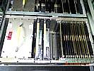
5245 CPU box 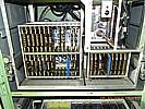
5246 Intercept computer controller interface 
10759 Expansion box cover with component list 
10763 CPU box cover with component list 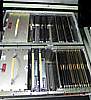
top two images stitched
missing image sections made black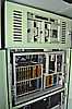
BC Van Intercept Comp Controller & Floppy Disks 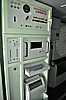
BC Van Intercept Comp Power Supply Bay 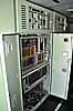
BC Van Intercept Computer Bay 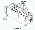
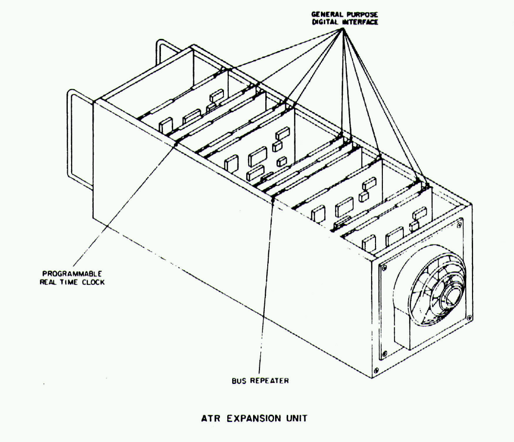
ATR Expansion Unit Exploded View 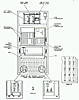
Intercept Computer Control Group Exploded View 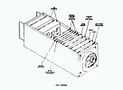
CPU Chassis Exploded View
from "Computerworld" December 20, 1976
Militarized Mini From Norden
Norwalk, Conn. - The PDP-11/34M fron the Norden Division of United Technologies Corp. is a militarized digital minicomputer compatible with the Digital Equipment Corp. PDP-11, according to the vendor.
Features PDP-11 Compatibility
The ruggedized mini features an extended instruction set with more than 400 instructions, the ability to perform single- and double-operand instructions, a memory expandable to 128K words, 900 nsec cycle time in core, byte parity, memory management, hardware multiply and divide and a floating-point option, the vendor said.
It can operate in environments from -65degrees F and in altitudes up to 85,000 feet, Norden said.
In addition the unit car withstand vibration, shock and humidiity: it meets the requirements of the MIL-E-5400, 16400 and 4158 specifications, the firm added.
A basic one-half chassis PDP-11M costs $15,200 to $20,200 depending on configuration; the full-chassis system costs $18,500 tp $24,700.
A system with 32K of memory and a communications interface ranges in price from $28,000 to $37,500. Norden said from Helen St., Norwalk, Conn. 06856.from "Computerworld" September 18,1978
Military Okays Norden PDP-11s
Norwalk, Conn. - Norden Systems's PDP-11-11M family of minicomputers has been given the U.S. military nomenclature designation of AN/UYK-42(V).
This designation is used as official recognition for all armed forces applications and was designated by the U.S.Naval Electronic Systems Command, Department of the Navy.
Norden Systems, a subsidiary of United Technologies Corp., militarizes the Digital Equipment Corp. family of PDP-]7 minicomputers under a special license.
Included in Norden's s militarized minicomputers are the PDP-11/70M, the PDP-11/-34M and the LSI-11M microprocessor. All have complete software identical to DEC's commercial software.In the late 1970's a digital computer was made available for the Nike. These were sent to "off-shore" locations as all U.S. sites had been de-activated. It is quite possible that this computer was a Norden PDP-11M. This was a licensed version of the DEC (Digital Equipment Corporation) PDP-11 that was housed in a tougher case and made more vibration resistant and in other ways made more suitable for a military environment.
It is known that the file system format on the floppy disks was RT-11M. (I have two floppies reported to be from a Nike site, but cannot figure out the data/program.) It had two 8 inch floppy disk drives, a printer, (and some I/O cards). As as best I can determine, the tracking antenna potentiometers were retained - the analog voltages being converted to digital for digital computing. Maybe the same for the range pot??
Any information about a digital Nike much appreciated.
Here is Rolf Dieter G�rigk's preliminary message - more info to follow:
August 2012, Rolf sent the following
The following web site and pages are no longer available on the Internet.
Archive.org does not have them archived due to Rolf's "robots.txt" string in each web page.
If anyone has recent information about Rolf or the contents of his web site, please send the information to me. Attempts to contact Rolf by several people have failed :-((
you`ll find the digital modifications under:
http://www.nikesystem.de/Pages/nike_content.html

Click on the "BCT & RCT" or "RADAR" button.

Most of the BCT modifications are at:
http://www.nikesystem.de/Pages/Equipment/nike_equipment_start.htm

Click on "New BCT" or "RCT"
Remember that the system was not modifyed to a full solid state status.
So some "old" parts were left in the system.

To look at the "radar" modifications click on the RADAR button:
http://www.nikesystem.de/Pages/Antennas/nike_radars.htm

You`ll find digital parts under "LOPAR", "HIPAR" or "TRACKING RADARS".
Often old & new (digital)  Parts are shown on the same page.
(Note the text.)

I`m working on better (Full HD) picture shows but that will take some time.

Hope that`s of some help!

Rolf D. Goerigk
In August 2012, wo Enzo Chieregatti < chrnzo @ libero . it > sent the following:
Donald Kraus < dkraus12 atsign hotmail dot com > e-mailed May 02, 2013
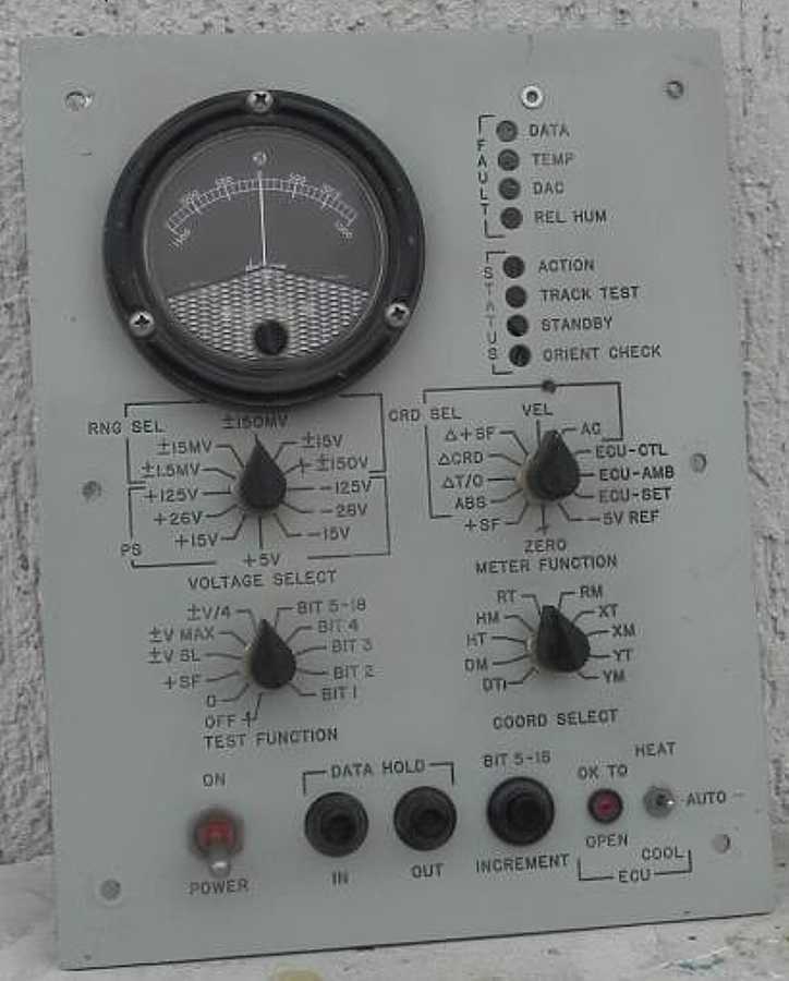
Hi I'm looking for information of the function of the Panel shown in the attached photo that was mounted in the nike system.Thank you
The photo panel was a converter analog-digital data between advancement station (R.S.P.U.) and the computer before changing years 80 is it possible?
Thought I would tell you a story that relates to the panel that one of your contributors asked about {above} When I was getting out of engineering school in 1978, I was working for a company in Buffalo, New York named Sierra Research.
By the way, this is the same company that built the zero set switches that you have pictures of on the same page. The circuit boards have the Sierra federal company code (12115) and some of the potted transformers actually have the Sierra Research name on them. The way the part numbers worked at Sierra was that the first two digits of the first group of four digits was the year of the contract that the part was for. The second two digits for circuit boards and things that were developed that were contract specific were the contract number for that year. For special part, like the transformers, other codes were used. The circuit cards for the zero set switch all have 6900 as the first four digits - meaning that these were designed for the first contract in 1969. Way before I joined the company. But this should help you place when the motor driven zero set switches were replaced with the electronic version.
Anyhow, the story about the digital to analog converter panel in the picture. The panel was part of a modification to replace the range and angle pots with microprocessors. The RSPUs (Radar Signal Processing Units -one for the MTR and one for the TTR) were mounted in the cabinet where the original range pots lived in the radar van. The original range pots were no longer used, the return video being processed by some fast digital logic coupled to an 8080 microprocessor. The angle pots were modified to remove the sine and cosine potentiometers. These were replace with an 8 pole resolver mounted directly on the 9:1 shaft of the pot. This resolver signal along with an existing 1:1 resolver signal were fed into converters in the RSPUs and another 8080 computed the pointing angles from resolvers along with the sine and cosine of the azimuth and elevation. Another microprocessor in each RSPU (we are up to six now - but they were only operating at 2.0 megahertz) combined the range and angle data to compute the various things that the original analog pots computed - slant range, X and Y along with the velocities of these things. A single microprocessor in one of the RSPUs (that would be number 7) then packaged this all for a data link to the battery control van, via a single coax cable.
The panel that you show was on the other end of the data link. This box contained a temperature controlled compartment (ECU - heater/cooler switch lower right) which contained an 18 bit multiplexed digital to analog converter. The converter also included ramping between the updates by use of the velocity components computed in the RSPU. The output of the converter was fed into the original analog computer. The velocity ramps were needed to help keep the digital sampling noise out of the analog circuits.
These modifications were performed on many of the Nike sites in Germany around the 1979/1980 time frame.
Anyhow, as a young engineer, I learned a bunch from helping put this equipment together. The documentation on the various signal flows along with the schematics of the radar equipment was top notch from my point of view, the organization of the actual equipment in racks and drawers supported trouble shooting even in a small space. A truly complex piece of equipment that was modularized to be maintainable. Not much that I have worked on since has come close to this.
Just thought I would give you some of the story on that panel.
Anyhow, hope this finds you well, and thanks again for the wealth of information on your site.Don Kraus


5) Solving the Predicted Intercept problem
To keep flight times down, (and increase the effective range) the missile is aimed ahead of the target at a calculated Predicted Intercept Point. If the aircraft flies a straight line, the missile horizontal flight path will also be straight. (A dog chasing a target runs directly toward the target, involving a longer run if the target runs straight.)
A person can worry that assuming that airplane flying straight might not be a good assumption, but what better can you make? One can wonder about the 10 million year success of dog-like creatures running directly toward the present position of their intended prey. However their prey can change direction and percent speed much faster than an aircraft. Dog chase path succeeds with a slightly different problem.
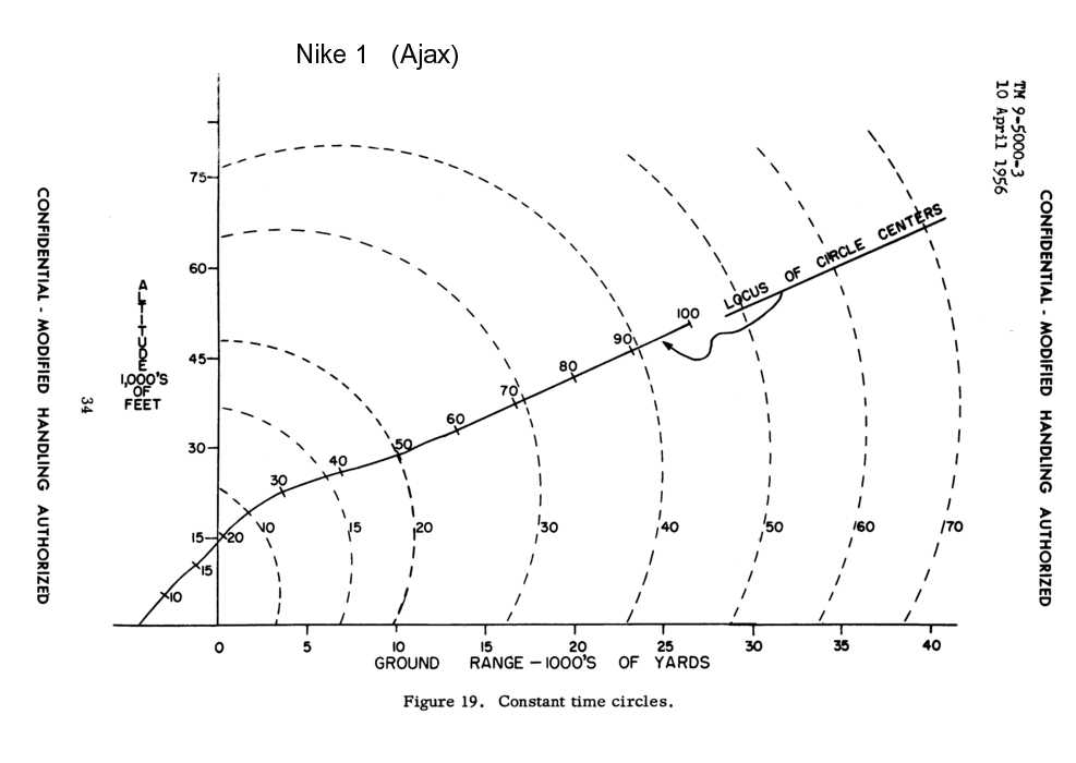
The computer has built into it average flight times to various ranges and altitudes. Here is a chart of
This information is compared with the speed and direction of the target until a valid time of flight to predicted intercept point is computed. This information is presented to the battery commander on the About the Nike Plotting Boards to assist him in making the firing decision.

Ajax Constant Time Circles
Ajax time of flight chart.The computer computes the Predicted Intercept Point by:
- Assuming the designated, tracked Plane will continue on its present course.
- Using a Trial Missile Flight Time, the position of the plane at the end of that time is estimated
- Using the same Trial Missile Flight Time, and a trial missile azimuth, the postion of the missile at the end of that time is estimated
- Based upon differences of estimated tracked plane position and missile position,
- the Trial Missile Flight Time is changed,
- the Trial Missile Azimuth is changed- Go back to step 2, do this continuously.
How Predicted Intercept Point is computed.
Rod Brimhall has a more complete discussion, 240 KBytes, .pdf
At longer ranges (flight times) the Predicted Intercept Point can vary greatly due to target aircraft maneuvers. The battery commander must make allowances for many possibilities.
The predicted time to intercept is also continuously updated during the missile flight to update the predicted intercept point to assist in making steering command commands.

 How Predicted Intercept Point is computed.
Please note: for a missile perspective, please see Nike Missile Flight Sequence
The missile is launched almost straight up, boosted to about mach 1.7 in 3.4 seconds. It then turns its belly toward the calculated Predicted Intercept (1 second), and a 7 g dive command is sent to the missile.
This is an image of the "Time-to-Intercept vs Altitude" plotting board describing the "Dead Zone" options which are limits of the Nike Flight dynamics. (The Nike is limited to a 7 g turn.) The Nike cannot get into the "Dead Zone" of altitude vs time. There are two options of systainer motor start depending upon how close the Predicted Intercept Point is to the launcher.
a) If the Predicted Intercept is close, the firing of the systainer motor is delayed, the missile goes slower, can turn tighter, with a smaller "Dead Zone" b) Normally the sustainer is started immediately after the booster falls away, faster flight larger turning radius, larger "Dead Zone".
The missile must not fly directly over the Missile Tracking Radar (MTR) because of limitions inherent in that type of antenna mount and the pointing system. To avoid flying directly over the MTR, special circuits are included in the computer to fly the missile in a path skirting around a flight path over the MTR. This situation is normally avoided by placing the launching area toward the expected direction of enemy aircraft - but the battery can be effective in any case.
A full dive command (7 g's) is sent to the missile to dive it from vertical toward horizontal. When the missile has reached a vertical angle that will be a good (1/2 g) flight path to the intercept point, the full dive command is removed and normal steering begins. For a preview of the "good flight path", jump ahead to End of 7 G dive .
After the 7 g dive, the computer flies the missile on a 1/2 g flight path to the predicted intercept point. For further details of the 1/2 g flight path, see page 64 of TM9-5000-3 (4.5 MBytes).
The predicted intercept point is constantly being updated by the computer from data from the target tracking radar and the missile tracking radar. Using the missile position from the Missile Tracking Radar, missile velocity and attitude generated in the computer, and the Predicted Intercept Point, the computer generates analog steering commands in gravity units (g's) for the missile. These commands are sent to the Missile Tracking Radar, where the analog commands are converted into radar pulse sequences indicating the command to the missile.
About 0.1 seconds before the missile will be closest to the target, a missile burst command is send by a coded pulse sequence to the missile by the missile tracking radar. This burst command is decoded and the missile warhead exploded. The goal is to explode the missile just before (10 meters) the missile would impact (or be at the closest point with) the aircraft. This way, the expanding blast of fragements goes through the space where the target aircraft would be - giving maximum damage even if a near miss.

7) Steering Command Details
The steering commands are basically to climb/dive and turn left/right a given number of earth gravitational acceleration units (g forces of fighter plane fame). As an example, the computer might command the missile to turn right at a rate of 1.0 g's. The missile would adjust its fins to turn hard enough so that the left/right accelerometer would indicate 1.0 g's right.Actually the missile fins are 45 degrees from horizontal, and the accelerometers are also 45 degrees from horizontal. The last stage of the computer rotates the command so that a 1.0 g right command will be sent as 0.707 g up/right and 0.707 g down/right which will result in 1.0 g turn right. You do remember your high school trig - don't you? Oh yes, you must be a "rocket scientist".
The missile steering commands are sent in analog form to the Missile Tracking Radar electronics where they are converted to radar pulse pairs which are received by the missile. For a description of the commands as they are sent by the Missile Tracking Radar see Missile Tracking Radar.
About 0.1 second before intercept, a burst command is sent to explode the missile and hopefully disable the target.
8) About the Nike Plotting Boards
There were 2 plotting boards
- Horizontal Plotting Board, with 2 pens
x,y - scale = +- 200,000 yards
- one pen always plotted the target
- the other pen plotted
- predicted intercept until the missile is launched
- missile position after missile is launched
- Altitude Plotting Board, with 2 pens
z,t - scale 0-100,000 feet, 0-160 seconds
- the left pen plotted the target altitude vs. time to intercept
- the right pen plotted time to intercept vs.
- predicted intercept altitude until the missile is launched
- missile altitude after missile is launched
There were timing marks every 10 seconds. These were quick jogs up and right.
A launch (fire) mark was a quick jog down and left.
The horizontal plotting board had lights to identify which pen was plotting what.
For a photo of the plotting boards, go to Battery Commander's View of the World.
9) How does the computer know the radar offsets?
The Target Tracking Radar (TTR) is considered the center of the world, well at least as far as the computer and IFC people are concerned. All distances are measured from the TTR. Plotting board distances and elevations are relative to the TTR.The computer must know where the Missile Tracking Radar (MTR) is relative to the Target Tracking Radar (TTR), and also the relative location of the Target Ranging Radar (TRR) relative to the Target Tracking Radar (TTR). This permits the computer to subtract out the positional differences, so that all three radars are, for computational purposes, located at the same point is space.
The offsets of the MTR and the TRR are dialed into potentiomenters located on the computer. The coordinates are as North/South, East/West, Up/Down from the Target Tracking Radar. Any errors dialed into these potentiometers will cause errors in flying the missile to the exact position of the target.
The positional differences of the various acquisition radars are not important because they are always within 50 yards of the TTR and errors in range and parallax due to this offset do not affect operation (primarily the locking on to the designated target by the TTR operators). It is important that the acquisition radars and the TTR (and any area supervision radars) have the same "North" reference to within about a degree for more exact target designation. (Which target is it?)
The Tracking Radars have the same North very precisely due to their alignment procedures.
10) Gotta have a little fun - Mechanical computers.
You have been very good students - serious - no sleeping or whispering - taking notes- ready for a quiz? I haven't the heart - time for fun.
Tim Robinson makes analog computers for fun - out of Meccano building "blocks".a differential analyzer a mini-Babbage machine difference engine
11) The Surface to Surface mission/mode
In July 2013, CW2 Robin E. Smith reminded me that there is not much discussion of the Hercules surface to surface mode.
OK - here goes what I can glean from the manuals ( way after my time ).Attack surface targets below the radar horizon. Dive straight down on a stationary target. The burst order causes guidance cutoff rather than an explosion.
Image from TM9-1400-250-10-2
Text from MMS 150, 1-P7
(3) Surface to surface mission. In a surface to surface mission (fig 7). the acquisition radars are not used because the target position is known. The range. azimuth, and elevation coordinates of the target are calculated and manually set into the TTR system. therefore, the TTR supplies constant target position data to the computer. Although the function of the computer system is similar to that described far a normal surface to air mission (a(1) above), the missile trajectory data must be manually set into the computer. This will, in turn, cause the missile to be guided toward a point in space above the desired point of impact. When the missile reaches the space reference point, the computer system issues a dive order that will cause the missile to approach the ground target vertically. As the missile approaches the ground, the computer sends a burst order by means of the missile tracking system. Due to special missile preparation in a surface to surface mission, however, the burst order does not cause the missile warhead to detonate. Instead, the burst order disables the missile fail-safe mechanism and causes guidance cut-off by disabling the missile receiver. The burst order also arms a preset barometric fuze in the missile warhead and rolls the missile 180 degrees to compensate for any possible control surface misalignment The missile then follows a vertical trajectory until the barometric fuze causes the nuclear warhead to detonate at a predetermined altitude above the target.
It doesn't take much imagination to figure that setting the TTR to a particular azimuth, elevation, and range, and firing a missile will cause the missile to get close to that point, and explode. Even in the Ajax program we thought that could be an interesting idea. If the point is outside the "dead zone", a circle about 10,000 yards from the launcher area, if you could see it, you could blast it.
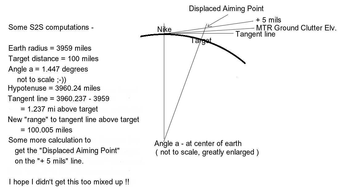
The Improved Hercules used a separate "Surface to Surface" mission/mode for both the computer and the missile. This enabled Nike to hit what it couldn't see - among other things, the curvature of the earth.
- There were formal instructions how to set up the TTR in azimuth, elevation, range from your map coordinates to the map coordinates of the target.
- To prevent the signal from the MTR being lost or distorted by ground clutter, the elevation angle was set to 5 mils above the MTR ground clutter at the TTR azimuth (above). The MTR could track and guide the missile reliably, and the burst command (which was not interpreted by the missile as burst but as "command guidance cut-off") would be reliably received by the missile
- A nomograph (NOT identical to this one) was available to aid calculations. Nomograph from http://www.tscm.com/rdr-hori.pdf
- CW2 Robin E. Smith was recognized as being expert in the above - I don't have the details of the computations.
"In preparation for our mobile mission each unit in our battalion had to prepare to calculate a surface to surface problem and set the radars and computer for firing. In the launching area there were also tasks to be completed, but they were fairly simple and the IFC personnel who calculated the fire mission gave them the information that the launcher crew had to set."- The missile was to be computer guided to be going "straight down" at burst signal time
- note: "straight down" near the earth 100 miles away is over 1 degree different
- CW2 Robin E. Smith said that "straight down" is relative to the target, not the Nike site.- The missile (before launch) was set into a special mode
- - a command burst was interpreted as command guidance cut-off
- - after command guidance cut-off, ??? missile guided internally along a 0 g path by its accelerometers ???
- - burst was to be triggered by altitude (atmospheric pressure) only
- - In Europe, a nuclear warhead was assumed?- Available manuals seem very vague about many useful and needed details - ? still classified ??
Some computations assuming the target is 100 miles from the Nike site.
Note that the tangent line from the Nike site is 1.24 miles above the target.
Please note: These calculation needs to be checked by some competent person.
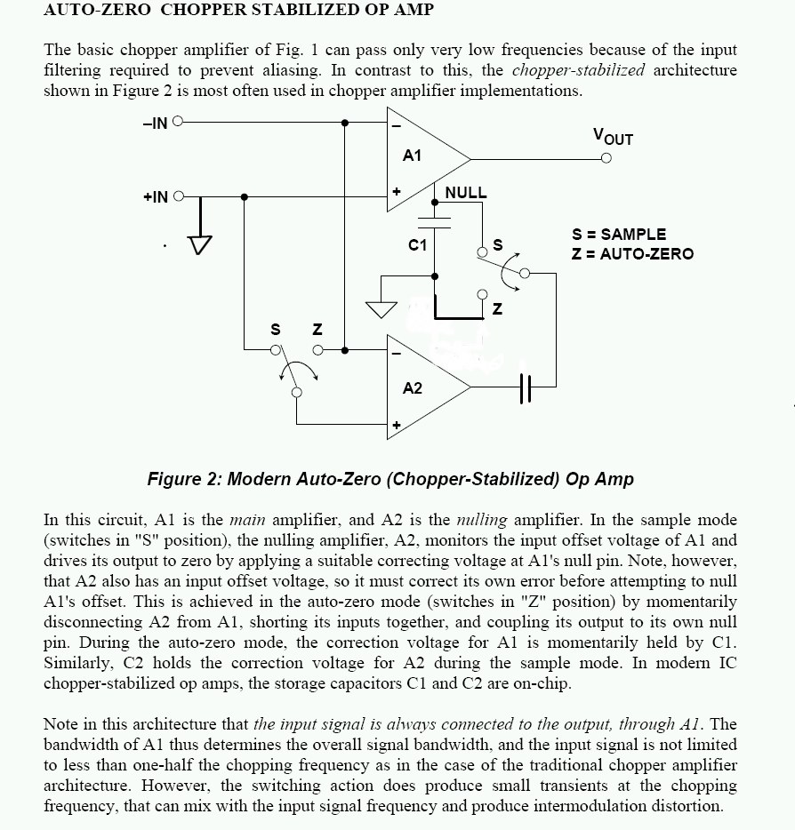
Appendix 1: Chopper Stabilized Operational Amplifiers (Op Amps)
Background
Operation
New (transistor) Zero Set Switch
Old (mechanical) Zero Set Switch
Background
It is very convenient to assume that Operational Amplifiers (Op Amps) for analog computers have - infinite gain (with stability) - no input "offset" voltages or currents Fortunately, they can be made very good so that for many problems errors can be held to less than say 0.01 percent per stage
- the "offset" current to the grid of a good triode (or FET) in on the order of nano amps. Unfortunately, efforts need to be made to reduce off-set voltage errors - An operational amplifier is expected to have zero volts output when the input is zero volts. Failure to do this is called "off-set error". Unfortunately, in real amplifiers, a large number of causes will cause voltage off-set errors which must be continuously corrected.
A principle method of correcting voltage off-set error is to use automatic Zero Set equipment which:
- reduces "offset" voltage - increases amplifier gain without decreasing stability You can manually zero set an operational amplifier by:
- removing the amplifier output from the circuit (no feed back) - connecting the input of the amplifier to analog ground (zero volts) - measuring to output voltage - adjusting the amplifier zero set to achieve zero volts on the output
then re-connecting the amplifier to the circuit for proper operationUnfortunately, temperatures, voltages and other conditions soon change, and you must zero set again, and yet again.
Fortunately, a good automatic method of zero setting operational amplifiers was discovered - just in time for Nike. - (leave the operational amplifier connected in the circuit :-)) - measure the voltage at the "summing junction", the input to the Op Amp - amplify this voltage by 200 (in the Zero Set Amplifier) ** if this voltage is excessive, a separate amplifier tube (in series) fires a warning neon lamp - apply this amplified voltage to the Op Amp zero set input
and do the above over and over again.The voltage measurement and correction can be done in the AC world - which makes life easier :-))
- Connect the input grid of the Zero Set Amplifier to ground
- Connect the output capacitor of the Zero Set Amplifier to ground
- The above steps, 1 & 2, provide a zero reference on the output capacitor
- Disconnect the output capacitor of the Zero Set Amplifier from ground
- Disconnect the input grid of the Zero Set Amplifier from ground
- Connect the input grid of the Zero Set Amplifier to the summing junction (Op Amp input grid)
- Connect the output capacitor of the Zero Set Amplifier to the Op Amp zero set capacitor
- The above 4 steps place a corrective charge on the Op Amp zero set capacitor
- Disconnect the output capacitor of the Zero Set Amplifier from the Op Amp zero set capacitor
- Disconnect the input grid of the Zero Set Amplifier to the summing junction (Op Amp input grid)
- Ready to start step one all over again
With careful design, this switch (and system) can be very reliable, well shielded, with low electrical noise.Further details about the Zero Set are in the Technical Manual TM9-5000-13-Ch04 Automatic Zero Setting Controls 155 KBytes
from another source
New (transistor) Zero Set Switch
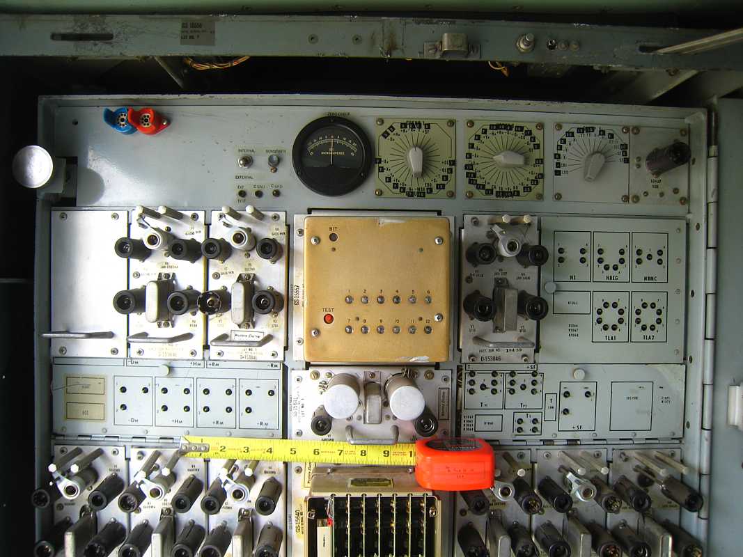
So - the Nike Analog Computer System
- this is one of four cabinets or racks -
includes Zero Set Switches (the brown boxes)
each can zero set 12 operational amplifiers.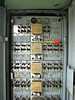
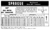
Transistor Style Zero Set Switch - Hercules only? introduced when? - Our Ajax system had "the old style" machanical below. I don't know how these "modern" circuits worked - The "3N93" are listed as "Dual Emitter Chopper Transistors" silicon PNP transistors
The brown box is a zero set switch, capable of zeroing 12 operational amplifiers. The chassis underneath is the Zero Set Amplifier, a gain 300 AC amplifier. 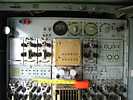
With the cover off, and one "dual line card" (my name) removed so you can see a typical socket. 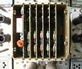
This is the component side of one of the six "dual line cards" (my name). Note the 3N93 transistors. 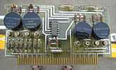
and the other side - mostly traces. 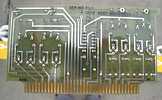
This is the component side of a "power supply card?" (my name) 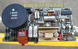
and the other side - mostly traces. 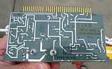
I'm not a transistor guy - if they don't have a heated cathode, they just can't possibly work ;-)) However, for you modern folks - who do believe in magic, here is a spec sheet - look for the 3N93. If anyone knows how the above zero setting circuits work - please send me the word.
Old Style (Mechanical) Zero Set Switch ? Ajax only ?


Appendix 2: Precision Gain Setting Resistors
We are familiar with the usual carbon composition and wire wound resistors, with the stated tolerances of 10% to 1%. These are not nearly accurate enough (nor stable enough) for gain setting resistors in a Nike system with a system error budget of say 20 feet in 25 miles between the errors of the two tracking radars and the various gain sensitive operational amplifiers in the computer.
just for the sake of argument, let us allow error budgets of:
- 7 feet to the Missile Tracking Radar subsystem - 7 feet to the Target Tracking Radar(s subsystem) - 7 feet to the computer subsystem
at a range of 25 miles.Friends, those are tight tolerances !! No room for slop anywhere - The gains of the Missile Tracking and Target Tracking radars in X, Y, and Height must be as identical (and correct) as possible.
An Op Amp gain is determined by the RATIO of the (feedback resistor)/(input resistor). [Assuming of course adequate amplifier gain.] If the feedback resistor is 0.1% low, the input resistor must be an identical 0.1% low. This correct and stable RATIO is attained by several paths:
- Careful precision matching during resistor network manufacture. This is done by selecting and trimming precision resistors monitored by a precision resistor bridge.
- Minimal changes in resistance due to temperature changes. This is attained by using wire wound resistors of low temperature coefficient metal - and non-stress packaging.
Packaging each resistor network so that each resistor is the same temperature as every other resistor in the packaged network. This is accomplished by placing the input and feedback resistors of each op amp into a separate aluminum container so that they get warm and cool together. A draft in the computer cabinet should affect all the resistors of an op amp "identically". The RATIO should be maintained.
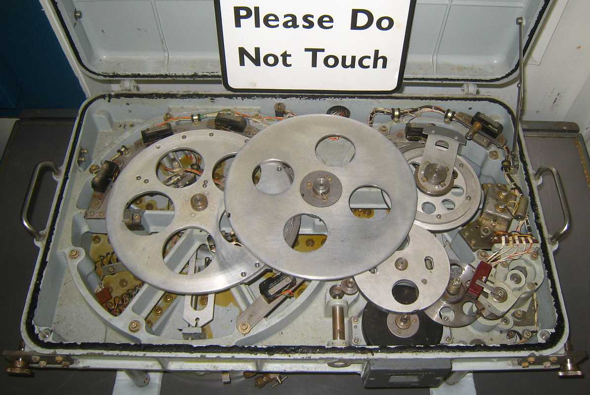
Appendix 3: Precision Servo-driven Potentiometers
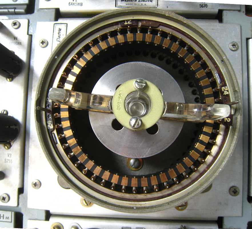
The general form of the potentiometer is a circular card, tapered to the math function, wound with resistance wire, contacted by a wiper arm. The Nike analog computer works in Cartesian coordinates coordinates ( X, Y, Z ) rather than spherical coordinates (elevation angle, azimuth angle, range).
Sin - cosine potentiometers are used in the target and missile tracking radar mounts to perform the conversions.
which are sent to the Nike analog computer.
- The slant range voltage is generated by each radar tracking radar system from the time delay from the magnetron pulse to the return echo (center of the "range gate")
- The elevation sin function converts slant range voltage into height ("Z"),
- The elevation cos function converts slant range voltage into ground range.
- The azimuth sin function converts ground range (above) into North|South ("Y")
- The azimuth cos function converts ground range (above) into East|West ("X")
The potentiometers in the Nike analog computer help with Time_To_Intercept, flight angle, flight characteristics, ballistic characteristics, ...
There are about 10 large precision servo-driven potentiometers in the Nike analog computer. These are contained in one of the 4 computer bays.
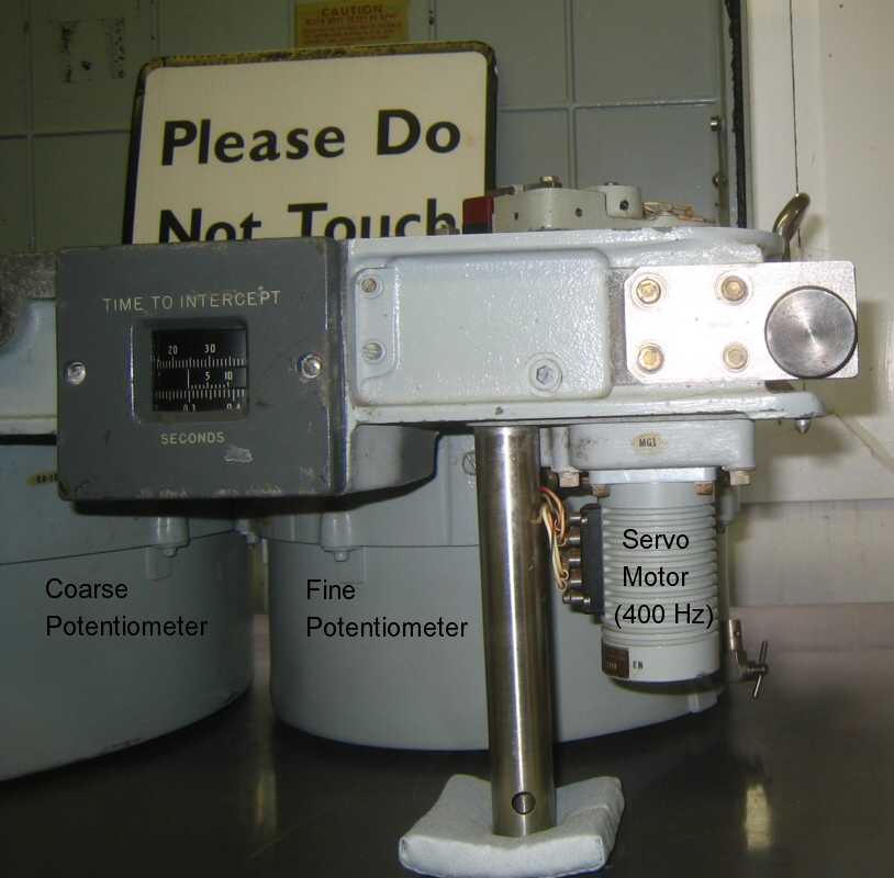
The Time_To_Intercept Coarse&Fine pots are in the second drawer from bottom
TM 9-5000-3 page 90 says there was a switch over from coarse time pot to fine time pot at 25 seconds to predicted intercept - all 7 functions -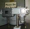
Time pots annotated - 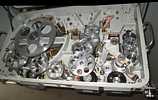
The bottom of four servo drawers, three functions in one box -
A visitor to SF-88, who lives in Los Angeles and taught at Ft. Bliss, says that these pots were used for nuclear warhead equiped Nike Hercules.

If you have comments or suggestions, Send e-mail to Ed Thelen
Return to Home, Return to beginning of Nike Computer, Goto Next Section
Updated February, 2022